Correlation, Causation, and Congress

The reddit site /r/dataisbeautiful too often has fun visualizations, but improper meaning derived from them. Some time ago, there was a post showing political donations to congress from the telecom lobby:

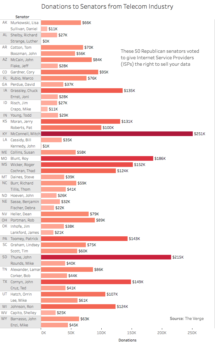
Clearly the context is to try and show that there’s a lot of money being dumped into congress in order to affect their thinking on votes pertaining to net neutrality. Is that really the case, though? In order to compare, we’d need the donations to all senators and compare.

The reddit user reformatted their plot as such using data from all senators:

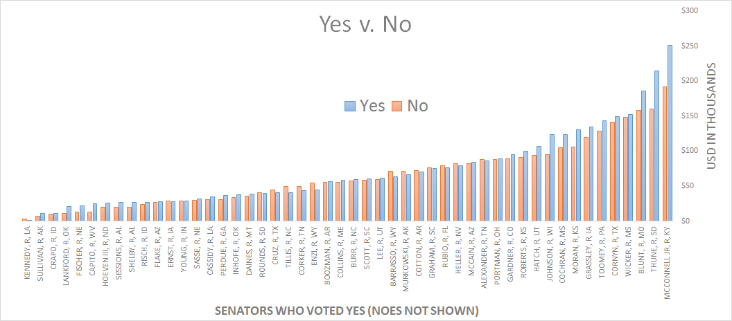
But still, the meaning here is lost. We see from the chart that there’s lots of senators, some receiving a lot more cash than others, but it’s hard to see if that has any effect on their votes at all. A better way to see if there’s any impact is to use a conditional inference tree and use their vote result as our response to model off of.

The data used for this exercise comes from this source, but for simplicity, I’ve included the raw table of data at the end of this post for ease of reproduction.

First, let’s just look at the distribution of cash split up by what the voting decision was:

 

votes <- read.table('clipboard', sep="\t", header=T)
votes$donations <- as.numeric(votes$donations)
boxplot(donations ~ vote
        ,data=votes
        ,xlab='Vote'
        ,ylab='Donation in $1000s'
        ,main='Voting Outcome By Telecom Donations in $1000s')

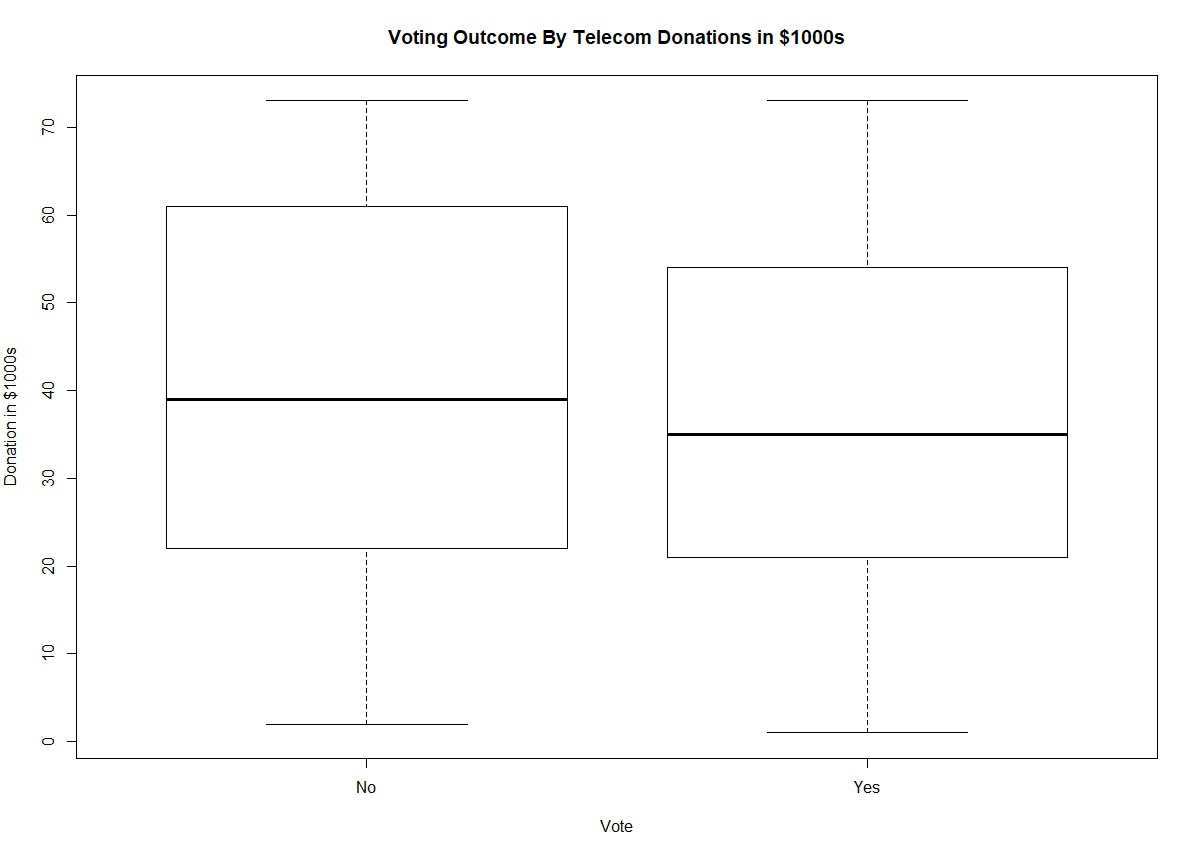
Now the above plot isn’t as sexy, but it’s a lot more useful. What we see is a distribution of data from the top down. The peak of the distribution in a box plot is the solid black line in the box, that’s where most of the data (the median) is. The interquartile range are the top and bottom of the box, and the whiskers outside the box show the maximum and minimum of those respective groups.

So what can we glean from that picture? Well we can tell that the yes votes had a lower median donation than the no votes. Oddly the opposite of what we were led to believe initially.

However, the data still has room to explore. How does political party come in to play in all this? The original thought was that there was a correlation between Republican votes and money. That doesn’t appear to be the case, in fact the opposite appears to be true. Seems like telecoms donating money to senators doesn’t necessarily dictate a vote in their favor.

We can extend this analysis with a conditional inference tree.

 

library(party)
votes.tree <- ctree(vote ~ . , data=votes)
plot(votes.tree, type='simple')

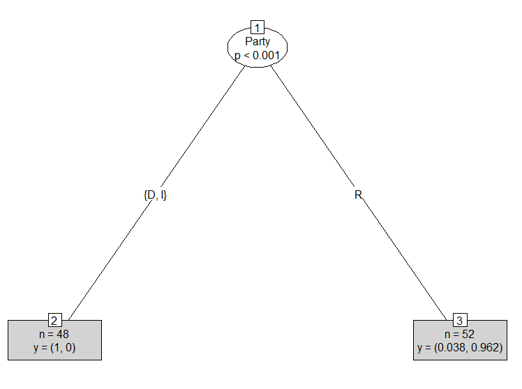
We read this plot as starting with the whole dataset, then splitting on party between D,I and R. For the D,I parties, we have a number of 48 data points (that’s what the n stands for), and a vector showing their percentage of no and yes votes respectively. In the case of the D,I party, we have a vector of y=(‘no’, ‘yes’). That means the D,I party had 100% no votes. On the other side of the aisle, we have n=52 republicans voting 96.2% yes and 3.8% no. That shows a much bigger impact of the vote than money does.

Sometimes the perceived beauty of the plot hides the real information of it. It’s always a better idea to show the meaning first, then gussy it up with all sorts of bells and whistles. If your visualization has no meaning behind it, you’re just window dressing.

Raw Data:

Senator State Party donations vote
ALEXANDER TN R $86 Yes
BALDWIN WI D $27 No
BARRASSO WY R $63 Yes
BENNET CO D $158 No
BLUMENTHAL CT D $148 No
BLUNT MO R $186 Yes
BOOKER NJ D $55 No
BOOZMAN AR R $56 Yes
BROWN OH D $57 No
BURR NC R $59 Yes
CANTWELL WA D $13 No
CAPITO WV R $25 Yes
CARDIN MD D $50 No
CARPER DE D $88 No
CASEY JR PA D $94 No
CASSIDY LA R $35 Yes
COCHRAN MS R $124 Yes
COLLINS ME R $58 Yes
COONS DE D $89 No
CORKER TN R $44 Yes
CORNYN TX R $149 Yes
CORTEZ MASTO NV D $10 No
COTTON AR R $70 Yes
CRAPO ID R $11 Yes
CRUZ TX R $41 Yes
DAINES MT R $39 Yes
DONNELLY SR IN D $11 No
DUCKWORTH IL D $13 No
DURBIN IL D $79 No
ENZI WY R $45 Yes
ERNST IA R $28 Yes
FEINSTEIN CA D $59 No
FISCHER NE R $22 Yes
FLAKE AZ R $28 Yes
FRANKEN MN D $76 No
GARDNER CO R $95 Yes
GILLIBRAND NY D $82 No
GRAHAM SC R $75 Yes
GRASSLEY IA R $135 Yes
HARRIS CA D $24 No
HASSAN NH D $7 No
HATCH UT R $107 Yes
HEINRICH NM D $29 No
HEITKAMP ND D $34 No
HELLER NV R $79 Yes
HIRONO HI D $29 No
HOEVEN III ND R $26 Yes
INHOFE OK R $38 Yes
ISAKSON GA R $58 No
JOHNSON WI R $124 Yes
KAINE VA D $20 No
KENNEDY LA R $1 Yes
KING JR ME I $20 No
KLOBUCHAR MN D $120 No
LANKFORD OK R $21 Yes
LEAHY VT D $129 No
LEE UT R $61 Yes
MANCHIN III WV D $50 No
MARKEY MA D $41 No
MCCAIN AZ R $84 Yes
MCCASKILL MO D $192 No
MCCONNELL JR KY R $251 Yes
MENENDEZ NJ D $95 No
MERKLEY OR D $45 No
MORAN KS R $131 Yes
MURKOWSKI AK R $66 Yes
MURPHY CT D $36 No
MURRAY WA D $88 No
NELSON FL D $106 No
PAUL KY R $31 No
PERDUE GA R $37 Yes
PETERS MI D $30 No
PORTMAN OH R $89 Yes
REED RI D $31 No
RISCH ID R $27 Yes
ROBERTS KS R $100 Yes
ROUNDS SD R $40 Yes
RUBIO FL R $76 Yes
SANDERS VT I $3 No
SASSE NE R $32 Yes
SCHATZ HI D $91 No
SCHUMER NY D $141 No
SCOTT SC R $60 Yes
SESSIONS* AL R $27 Yes
SHAHEEN NH D $71 No
SHELBY AL R $27 Yes
STABENOW MI D $54 No
SULLIVAN AK R $11 Yes
TESTER MT D $82 No
THUNE SD R $215 Yes
TILLIS NC R $41 Yes
TOOMEY PA R $143 Yes
UDALL NM D $105 No
VAN HOLLEN MD D $55 No
WARNER VA D $160 No
WARREN MA D $20 No
WHITEHOUSE RI D $72 No
WICKER MS R $152 Yes
WYDEN OR D $71 No
YOUNG IN R $29 Yes

headline image used from salon.com