It’s obvious that my previous blog posts show that I’m a little obsessed with tabletop board games at the moment. Like all people waist deep in their hobby, I’ve been having to steady myself multiple times in the Amazon shopping cart thinking “hmm…am I really interested in this game, or is it just that I’m riding the hype train?”
Like all good data scientists, I decided to experiment on myself. How do my interests in these games change over time? Am I really that interested in this game now as I am maybe a week from now?
This is a question that can be answered many different ways and the analysis presented here can be abstracted to any product in particular. I’d be curious if others have done user research in this domain what their thoughts are.
In 2017 I did an experiment that whenever I was interested in a game (watched a youtube video, looked up rules info, etc) I added 1 to a count next to the game so I could keep a tally of which ones I was most interested in.

2017 titles I was most interested in. No date data here to play with, unfortunately.
The distribution is, as you’d expect, long tailed with a few games having the most interest. Of 80 or so games I was interested in 2017, only 28 had an interest value greater than 1. Long tailed indeed! This data doesn’t really tell us much, though. How did my interest change throughout the year? How interested am I in Dominant Species now compared to 6 months ago?
To answer those kinds of questions, I went back to the drawing board. For a given day, if I was interested in a game, I’d record the date and the name of the game I was interested in. The goal here was to show how the interest accumulates over time.
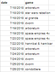
2018 data structure. Simple, but a lot of power can be drawn from this with the right mindset.
The full dataset for this can be found on my GitHub here. What’s important about this data is that, not only can I repeat the same kind of analysis I did last year for a “top 10 most interested games” list, but just having the data broken out by date allows so much more analytical power.

The 2018 data set allows me to back into the same form of results I got for 2017. Space Empires, Hannibal, and Dune still rank high in the top 15 for 2018.
Let’s see how this data looks like with a running cumulative sum over time:
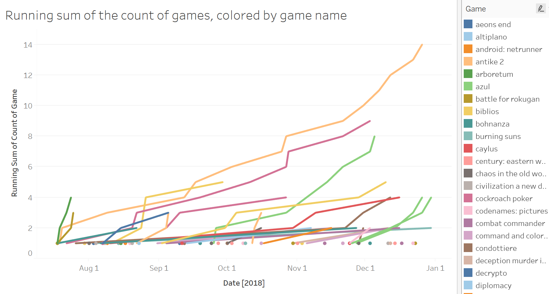
Tableau does these kinds of graphs in a slightly weird way, but it gets the point across. The highest orange line is Space Empires 4x and the magenta line beneath it is Hannibal & Hamilcar.
This view shows us that some games can have a very high growth rate in interest compared to others, and that some don’t have any more interest after a certain period of time. What we need to do is show relative interest by implementing a decay.
The Meh Factor

King Phillip the Fair gauges his own algorithmically-driven interest level when judging peoples castles in the game Caylus
The cornerstone to this analysis is asking “how does my interest in something decay over time?” My original thought was that my interest would decay linearly over time. For example: maybe my interest in game X is 25 on a certain day and that the next day it goes down to 24. But what happens when this hits 0 eventually? Does it go negative? I decided to keep things relatively simple and go with a percentage-based decay rate of 5%. So on a certain day, interest in game Z would go from 100 down to 95 then 90.25 the next.
From discussions I’ve had with some people in the field, there wasn’t an obvious paper they could point me to which definitively answers the question of what decay rate to use (if any). In the field of user research, I’m sure there’s a bunch of different variables that come in to play about time of year, type of product, how many times the person has engaged with the thing, etc. My simple approach of a 5% decay day-over-day might be too simple to be applied to an enterprise-level solution, but for this blog post I’m sure it’s a fine toy to play with.
The Interest-Decay Algorithm
Starting from the daily data above, the basic algorithm here is:
- Increase interest by 1 if a game’s name is present on a certain day
- Decrease interest by 5% if a game’s name is absent on a certain day
Putting this together in R is relatively straightforward:
library(dplyr)

log <- read.table("clipboard", sep="\t", header=T)
log$date <- as.Date(log$date, format = "%m/%d/%Y")

testdf <- data.frame(seq(min(log$date), max(log$date), by = "days"))
names(testdf) <- c("date")
test_join2 <- testdf

for(j in 1:length(unique(log$game))){

  game_subset <- subset(log, subset=(log$game == unique(log$game)[j]))
  test_join  1){
      test_join[i,3] <- (test_join[i-1, 3]) + 1 #interest addition
    }else{
      test_join[i,3] <- (test_join[i-1, 3]) * 0.95 #decay
    }
  }
  result_join <- data.frame(test_join$date, test_join$V3)
  names(result_join) <- c("date", as.character(unique(log$game)[j]))
  test_join2 <- left_join(test_join2, result_join, by='date')
The output for this code produces a column for each game and the rows range over the min and max dates from the raw data.
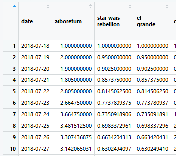
Model output: for each day that the raw data has a game name, it’s iterated up by 1. If that game isn’t present, we decay it by 5%.
Visualized Outputs
I’ve yet to figure out how to embed Tableau visuals into WordPress properly, so I’ll link to the Tableau Public visualization I have of the above output here. It allows us to look at various games and how the values look over time. Let’s take a look at one a few case examples:
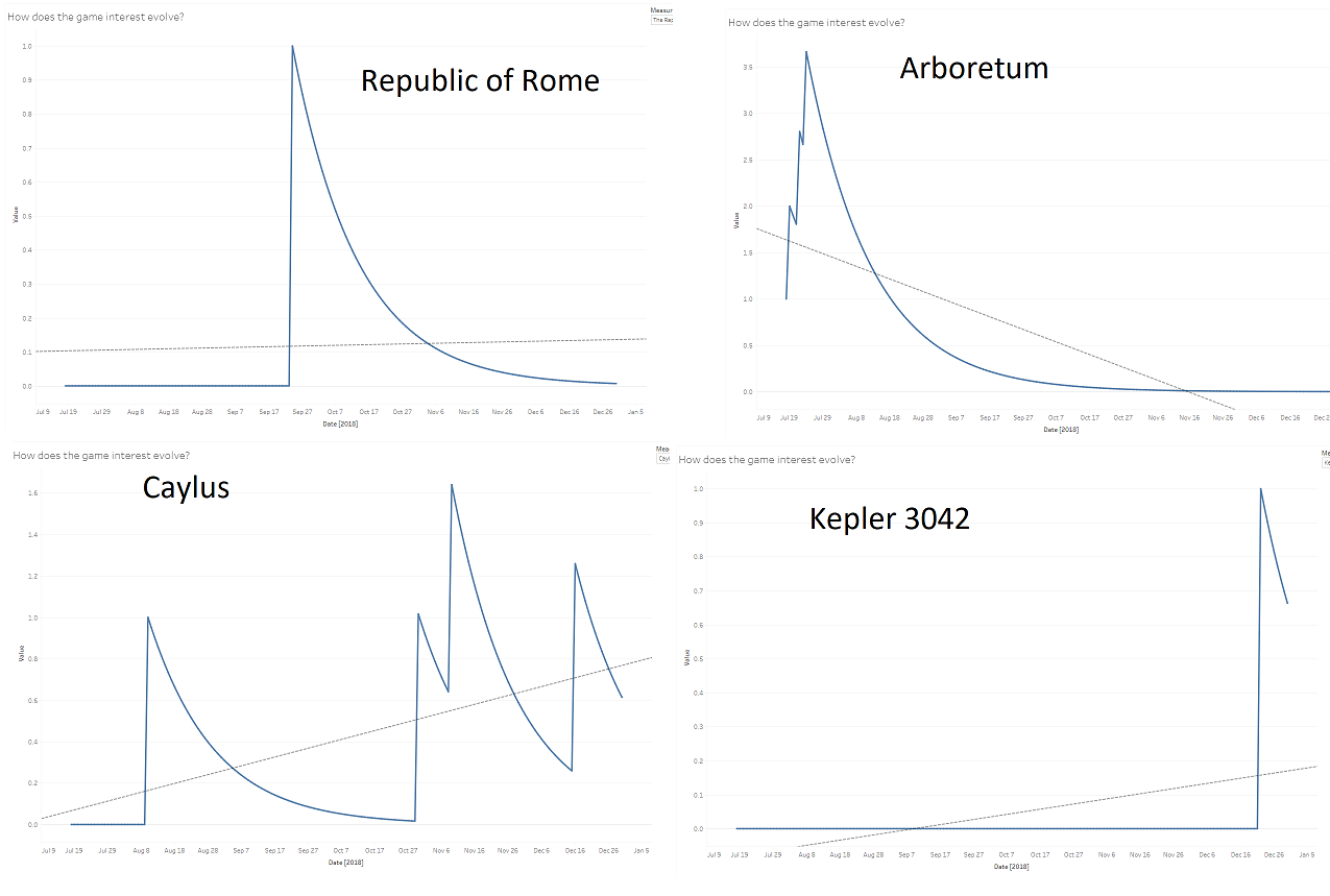
Four example games from the resultant data set.
These four examples show a lot of interesting behavior:
- Republic of Rome: many of the games in the resultant output are like this, where I was interested once and never really thought about them again.
- Arboretum: there are some games in the data in which I had a growing interest in, then eventually stopped recording interest. In the case of Arboretum that’s because I purchased the game right around the peak, so it makes sense why it wouldn’t show up again.
- Caylus: this is a game that I’ve been on-and-off interested in for a while. The accumulated interest pushes the fitted linear trend upwards showing that I have a growing interest in the game overall.
- Kepler 3042: this game I only recently heard about and was interested so I logged it. As you can tell, there’s a slight incline to the fitted trend line as a result. This is because the model fit in Tableau (which I’m using for visualization here specifically) is modelling over all the results for that slice of data, which is the entire range of the data set. Kepler only has a single data point of interest and all the ones prior are zero, so this would be a case of recency bias in the model.
What’s interesting next is to see how the top games I was interested in from the earlier picture model out over time. Let’s keep things simple and look at the top 6:
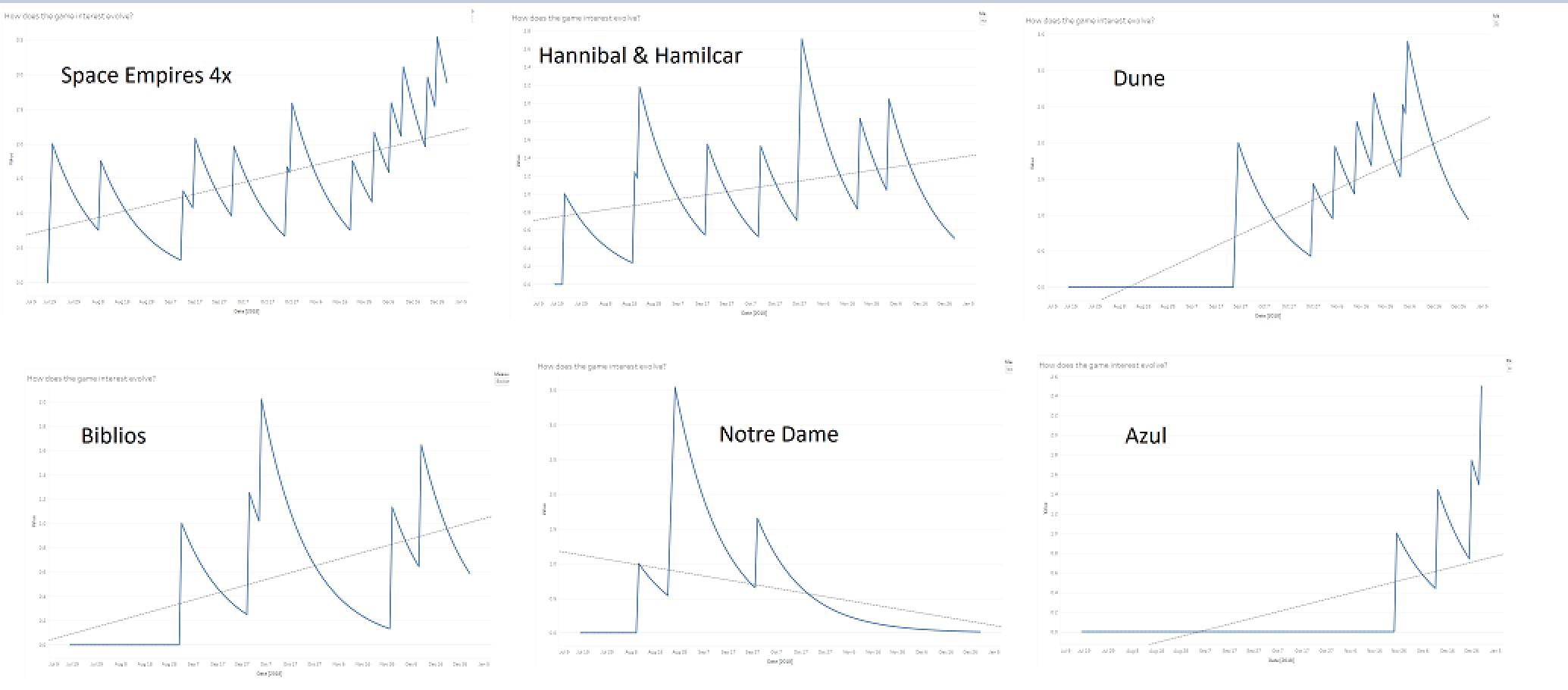
Top 6 games of cumulative interest for 2018 and how they model over time. Caveat: I’m including Azul here even though it’s #7 since we just saw #6 Arboretum in the last figure.
An interesting observation here is that They all appear to be increasing over time from the linear model fit that’s been applied except for Notre Dame, which appears to be trending downward. This begs the question: do I really have a sustained interest in that game compared to the others? Also: is the interest rate in Azul higher if we remove the 0 data before its first appearance?
To properly answer these questions I’m going to turn back to R.
Model Layering
Starting from the raw date-level data, I’m looking at just the time range for interest in which a game exists (ie first appearance until now) and fitting a linear model on that data specifically. Before we saw the trend lines being applied to the full range of date data available, which might not be fare to some more recent games than older ones of interest.
For this I’m only really interested in a few things:
- The slope of the fitted trend line
- How many total days has the game of interest been on my radar
- How many times has that game shown up in total
game_freq <- data.frame(table(log$game))

final <- data.frame(matrix(0, ncol=4))
colnames(final) <- c("game", "interest", "days on radar", "days of interest")

for(k in 2:ncol(test_join2)){

  model <- data.frame(test_join2$date, test_join2[,k])
  model_subset  0))
  coef <- (lm(model_subset$test_join2...k. ~ model_subset$test_join2.date))$coefficients[2]

  days_of_interest <- subset(game_freq, subset=(Var1 == colnames(test_join2)[k]))[2]

  final_1 <- data.frame(colnames(test_join2)[k], coef, nrow(model_subset), days_of_interest)
  colnames(final_1) <- c("game", "interest", "days on radar", "days of interest")

  final <- rbind(final, final_1)
}
This produces a table with the following form:

In this view we see that there are 8 games which have a positive slope on their fitted linear model trend line. Many of those have relatively few days of interest with the ones at the top having a relatively low amount of time in total being on my radar. This shows that this approach can be susceptible to recency bias or ‘cult of the new’ as it were.
Final Thoughts

A reasonably accurate summary of how I react to new games. Image credit to http://www.ibgcafe.com/news/the-cult-of-the-new/
Overall, I thought this was a fun experiment to see what more analysis could be done if I treated my data collection method differently. By switching to a date-based format instead of just an all-up one, I was able to extract a lot more interesting data out as a result.
The world of user behavior research is one that’s new but interesting to me. There seems to be a rich area of exploration in figuring out how a person’s interest in a thing changes over time as well.
By applying some linear model fits on the data, I was able to see that despite about half of it having a total interest above 1, only about 10% of the total data had any kind of positive trend associated with it.
There seem to be a lot of pitfalls involved with this kind of modelling, especially those related to recency bias. Being able to not have your data biased by something just because it’s new might be a difficult problem to wrangle.
Most importantly I think I need to play a game of SpaceCorp with someone…
featured image credit: https://www.uxpin.com/studio/blog/testing-redesigning-yelp-user-research-upcoming-e-book/
